Gauss Elimination Method Presentation

Introduction to Gauss Elimination Method
Gauss elimination method is a numerical technique used to solve systems of linear equations. It was developed by Carl Friedrich Gauss in the early 19th century. This method is widely used in various fields, such as engineering, physics, and computer science.	Image Source
		1

Steps of Gauss Elimination Method
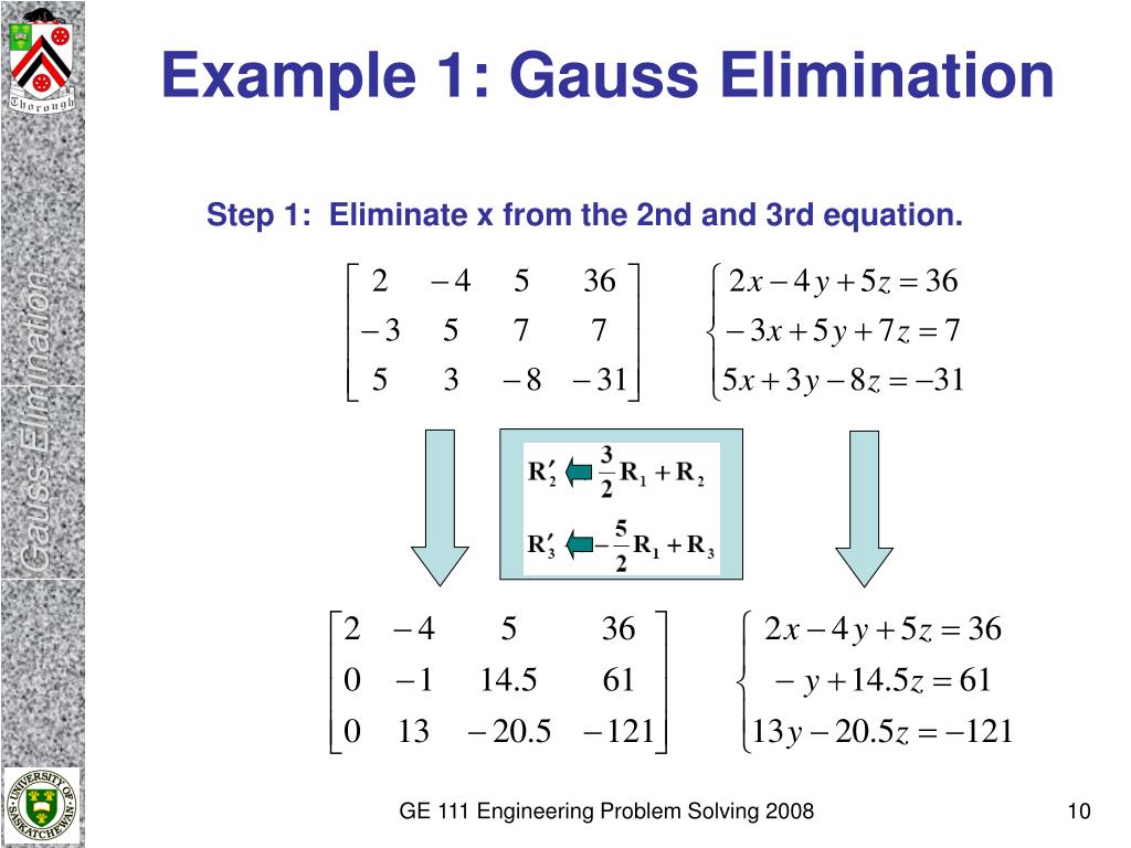
Step 1: Write the augmented matrix of the system of linear equations. Step 2: Perform row operations to transform the augmented matrix into row-echelon form. Step 3: Back-substitute to find the values of the variables.	Image Source
		2

Writing Augmented Matrix
The augmented matrix is a matrix that combines the coefficients of the variables and the constants of the equations. Each row of the augmented matrix represents an equation in the system. The last column of the augmented matrix contains the constants of the equations.	Image Source
		3

Row Operations
In Gauss elimination method, three row operations are commonly used: - Interchanging two rows. - Multiplying a row by a non-zero constant. - Adding or subtracting a multiple of one row from another row. Your second bullet Your third bullet	Image Source
		4

Row-Echelon Form
Row-echelon form is a special form of the augmented matrix where each leading coefficient (the first non-zero element in each row) is equal to 1. All elements below the leading coefficient are zeros. The leading coefficients form a staircase pattern from left to right.	Image Source
		5

Example of Row-Echelon Form
Here's an example of a row-echelon form: 1 2 3 | 4 0 1 -1 | 2 0 0 1 | -1 Notice how the leading coefficients are all equal to 1, and the elements below them are zeros. Your third bullet	Image Source
		6

Back-Substitution
After obtaining the row-echelon form, we can perform back-substitution to find the values of the variables. Start with the last row and solve for the last variable. Substitute the value of the last variable into the second-to-last equation and solve for the second-to-last variable.	Image Source
		7

Solving the System of Linear Equations
After back-substitution, we have the values of all the variables. We can write the solution as an ordered set of values for each variable. If the system has a unique solution, the Gauss elimination method will find it.	Image Source
		8

Advantages and Disadvantages
Advantages: - Gauss elimination method is straightforward and easy to understand. - It can be easily implemented in computer programs. - It is widely applicable to various types of systems of linear equations. Disadvantages: - If the system has infinitely many solutions or no solutions, the method may not provide a clear indication. - It can be computationally expensive for large systems with many equations and variables. - The method may suffer from round-off errors when dealing with floating-point arithmetic. Your third bullet
		9

Join the SlideMake Community